library(dplyr)
library(ggplot2)
library(tibble)
library(viridis)
library(RColorBrewer)

1 Introduction

This tutorial uses the built-in iris dataset to introduce core skills for working with data in R. Rather than focusing on abstract concepts, we will learn by exploring a real dataset step by step.

You will practice using dplyr to organize and transform data, helping you focus on the parts of the dataset that matter for your questions. You will then use ggplot2 to create clear and informative visualizations, building from simple plots to more detailed, multi-dimensional graphics with customized color palettes.

Finally, you will connect these visual patterns to statistical tests, learning how to formally evaluate differences and relationships in the data.

By the end of this tutorial, you should be able to:
- explore and summarize a dataset
- reshape and refine data for analysis using dplyr
- create effective visualizations with ggplot2
- apply basic statistical tests and interpret their results

The goal is not just to learn individual tools, but to see how they work together as part of a complete data analysis workflow.

1.1 Download this .Rmd file

Download RMD file

1.2 Read in the dataset

data(iris)

1.3 Inspect the data

head gives the top 6 rows of the dataframe

head(iris)

1.4 Check the Structure

str(iris)

## 'data.frame':    150 obs. of  5 variables:
##  $ Sepal.Length: num  5.1 4.9 4.7 4.6 5 5.4 4.6 5 4.4 4.9 ...
##  $ Sepal.Width : num  3.5 3 3.2 3.1 3.6 3.9 3.4 3.4 2.9 3.1 ...
##  $ Petal.Length: num  1.4 1.4 1.3 1.5 1.4 1.7 1.4 1.5 1.4 1.5 ...
##  $ Petal.Width : num  0.2 0.2 0.2 0.2 0.2 0.4 0.3 0.2 0.2 0.1 ...
##  $ Species     : Factor w/ 3 levels "setosa","versicolor",..: 1 1 1 1 1 1 1 1 1 1 ...

1.5 Get a Summary

summary(iris)

##   Sepal.Length    Sepal.Width     Petal.Length    Petal.Width   
##  Min.   :4.300   Min.   :2.000   Min.   :1.000   Min.   :0.100  
##  1st Qu.:5.100   1st Qu.:2.800   1st Qu.:1.600   1st Qu.:0.300  
##  Median :5.800   Median :3.000   Median :4.350   Median :1.300  
##  Mean   :5.843   Mean   :3.057   Mean   :3.758   Mean   :1.199  
##  3rd Qu.:6.400   3rd Qu.:3.300   3rd Qu.:5.100   3rd Qu.:1.800  
##  Max.   :7.900   Max.   :4.400   Max.   :6.900   Max.   :2.500  
##        Species  
##  setosa    :50  
##  versicolor:50  
##  virginica :50  
##                 
##                 
##

2 Basic `dplyr` summaries

2.1 Count number of entries by Species

In English: “take the object iris and then count the groups in the column Species”

iris %>%
  count(Species)

2.1.1 Compute average measurements by species

iris %>%
  group_by(Species) %>%
  summarise(
    n = n(),
    avg_sepal_length = mean(Sepal.Length),
    avg_sepal_width  = mean(Sepal.Width),
    avg_petal_length = mean(Petal.Length),
    avg_petal_width  = mean(Petal.Width)
  )

2.2 Filter rows

2.2.1 Look only at `setosa`

In English: “take the object iris and then filter to only include Species = setosa rows, and then show the top 6 rows”

iris %>%
  filter(Species == "setosa") %>%
  head()

2.2.2 Look only at flowers with large petals

iris %>%
  filter(Petal.Length > 5, Petal.Width > 1.5) %>%
  head()

2.3 Create new variables

In English: “Create the new object iris2 by starting with the object iris and then creating a new column with the name Petal.Area that is the value of Petal.Length * Petal.Width”

iris2 <- iris %>%
  mutate(Petal.Area = Petal.Length * Petal.Width)

head(iris2)

2.3.1 Create and Summarize

How do you say this in english?

iris2 <- iris2 %>%
  mutate(Sepal.Ratio = Sepal.Length / Sepal.Width)

summary(iris2$Sepal.Ratio)

##    Min. 1st Qu.  Median    Mean 3rd Qu.    Max. 
##   1.268   1.546   2.032   1.954   2.225   2.962

2.4 First ggplot: a scatterplot

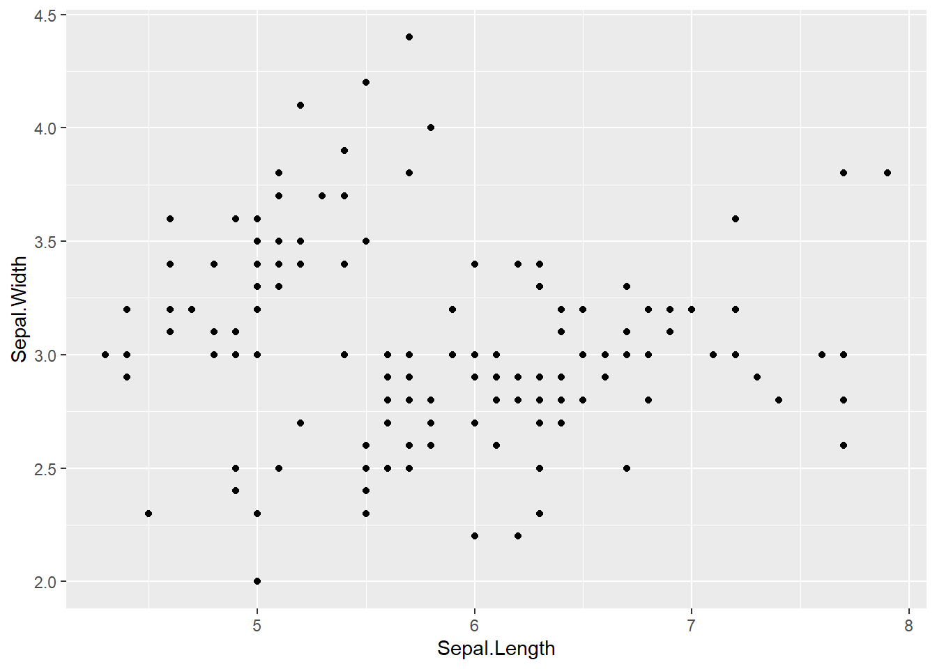
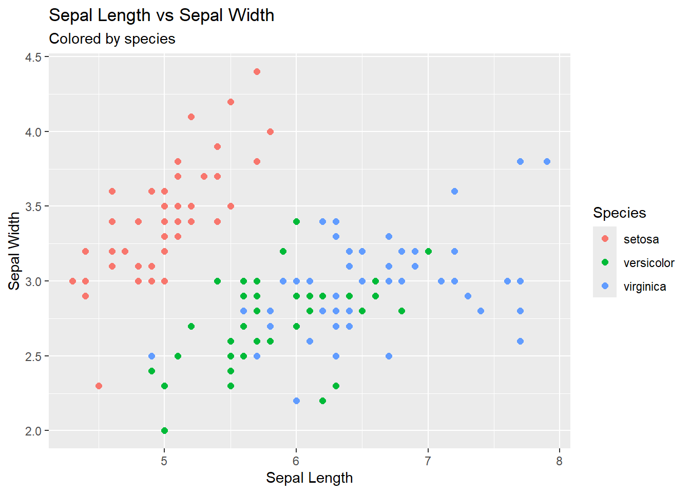
ggplot(iris, aes(x = Sepal.Length, y = Sepal.Width)) +
  geom_point()

2.4.1 Color by species

color = Species//Also adding custom plot labels

ggplot(iris, aes(x = Sepal.Length, y = Sepal.Width, color = Species)) +
  geom_point(size = 2) +
  labs(
    title = "Sepal Length vs Sepal Width",
    subtitle = "Colored by species",
    x = "Sepal Length",
    y = "Sepal Width"
  )

2.4.1.1 Color palette = `RColorBrewer`

ggplot(iris, aes(x = Petal.Length, y = Petal.Width, color = Species)) +
  geom_point(size = 2) +
  scale_color_brewer(palette = "Dark2") +
  labs(
    title = "Petal Dimensions by Species",
    x = "Petal Length",
    y = "Petal Width"
  )

2.4.1.2 Colorblind-friendly = `viridis`

ggplot(iris, aes(x = Petal.Length, y = Petal.Width, color = Species)) +
  geom_point(size = 2) +
  scale_color_viridis_d() +
  theme_minimal() +
  labs(
    title = "Petal Dimensions by Species",
    x = "Petal Length",
    y = "Petal Width"
  )

2.5 Multidimensional Plots

2.5.1 Going 4D!

x = Sepal.Length // y = Petal.Length // color = Species // size = Petal.Width

ggplot(iris2, aes(
  x = Sepal.Length,
  y = Petal.Length,
  color = Species,
  size = Petal.Width
)) +
  geom_point(alpha = 0.8) +
  scale_color_viridis_d() +
  labs(
    title = "A Multidimensional Plot",
    subtitle = "Color = species, size = petal width",
    x = "Sepal Length",
    y = "Petal Length"
  ) +
  theme_minimal()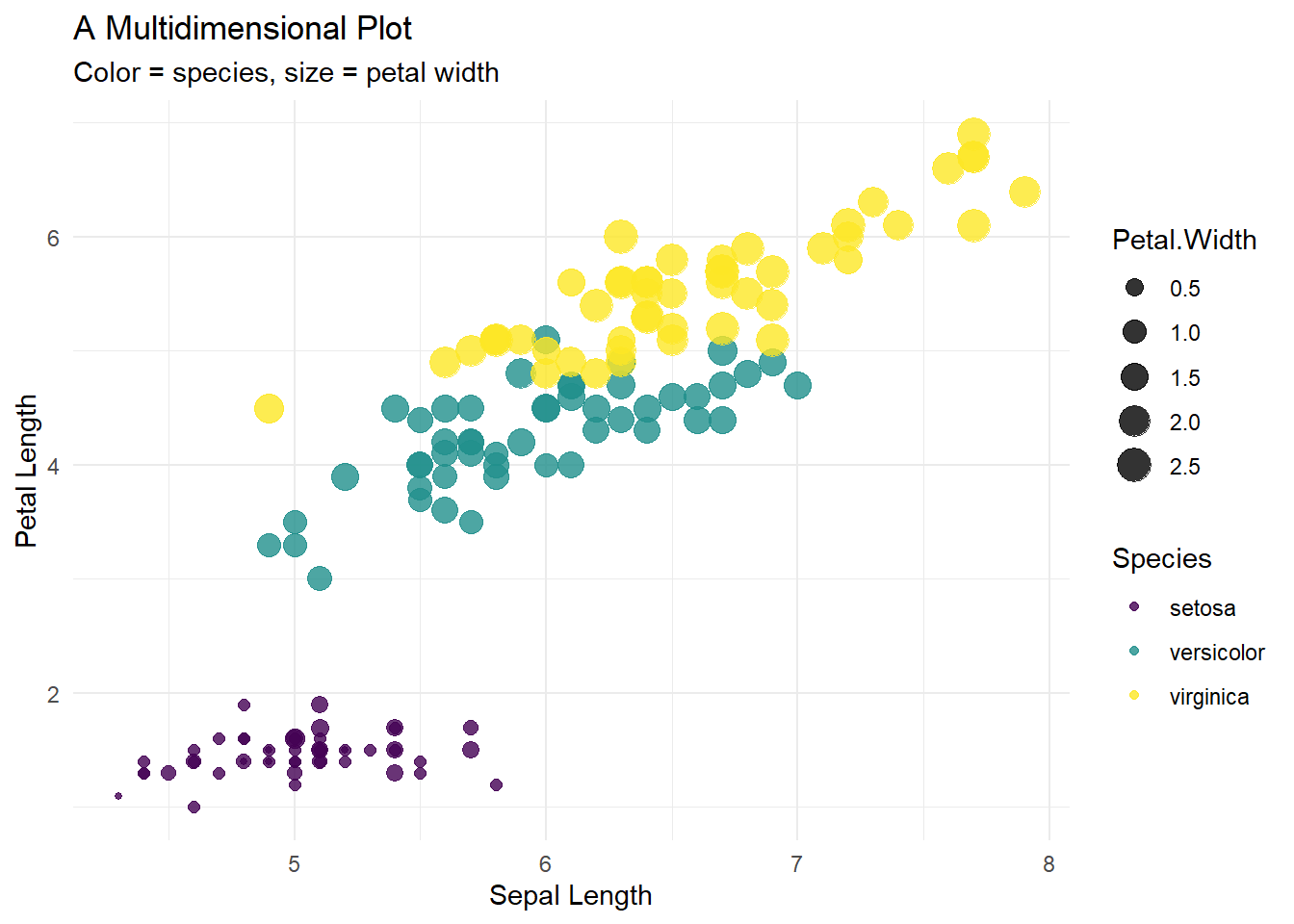

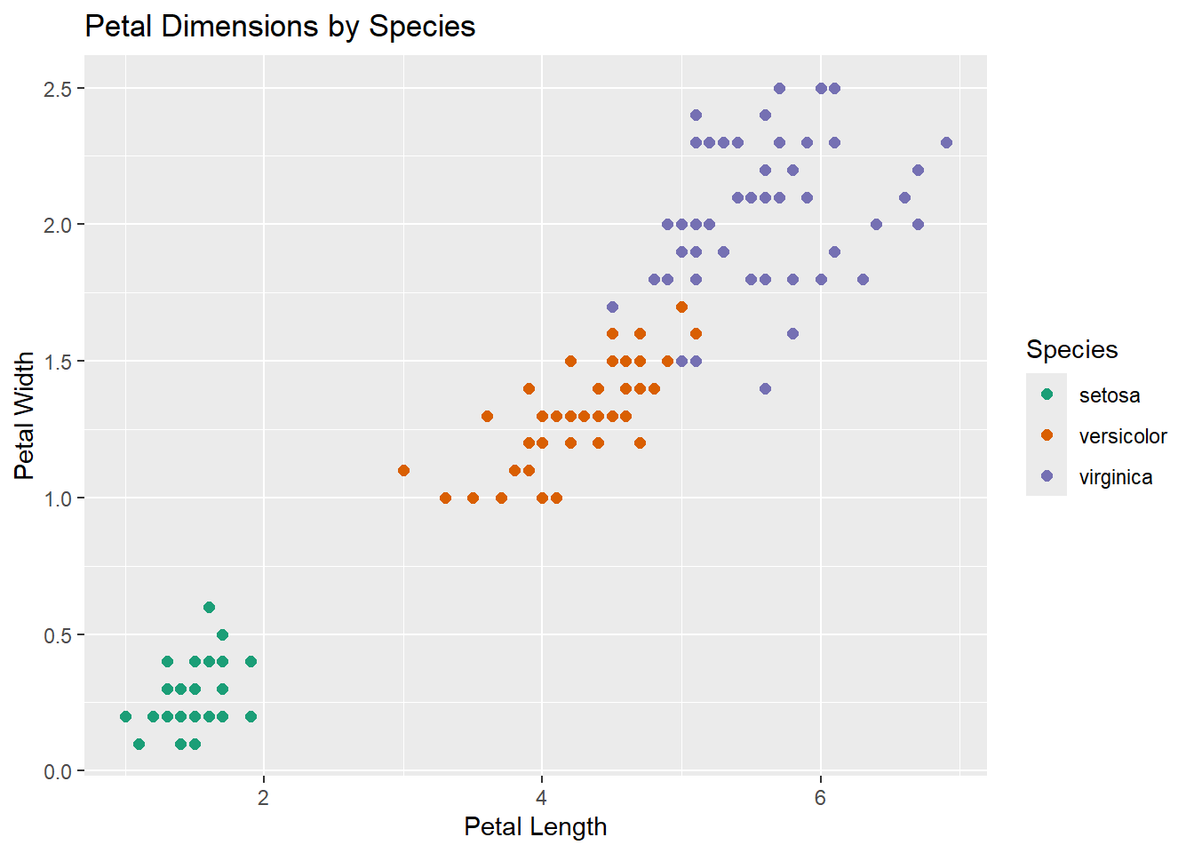
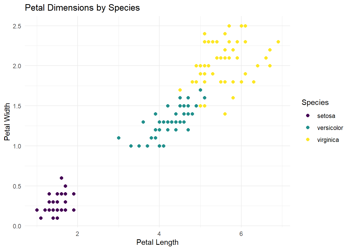
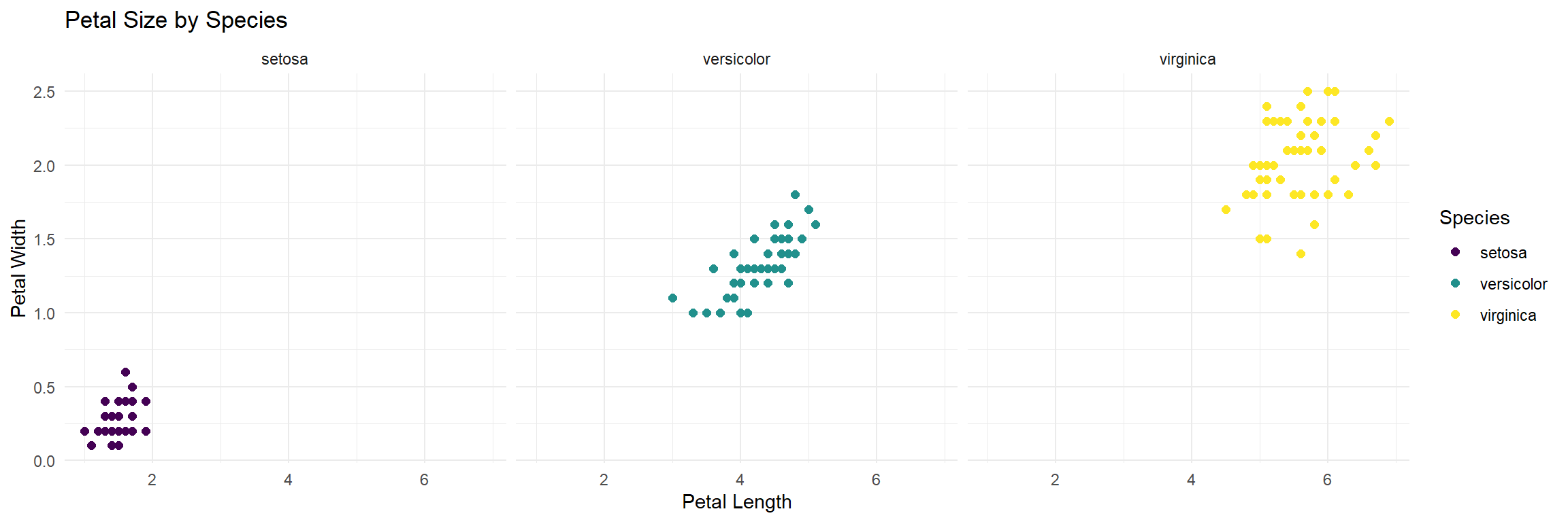
2.6 Faceting for comparison

facet_wrap(~Species)

ggplot(iris, aes(x = Petal.Length, y = Petal.Width)) +
  geom_point(aes(color = Species), size = 2) +
  facet_wrap(~Species) +
  scale_color_viridis_d() +
  theme_minimal() +
  labs(
    title = "Petal Size by Species",
    x = "Petal Length",
    y = "Petal Width"
  )

2.7 Summaries plus plots

2.7.1 Calculate the Summary

species_summary <- iris %>%
  group_by(Species) %>%
  summarise(
    avg_petal_width = mean(Petal.Width),
    avg_petal_length = mean(Petal.Length)
  )

species_summary

2.7.2 Plot the Summary

ggplot(species_summary, aes(x = Species, y = avg_petal_width, fill = Species)) +
  geom_col() +
  scale_fill_viridis_d() +
  theme_minimal() +
  labs(
    title = "Average Petal Width by Species",
    x = "Species",
    y = "Average Petal Width"
  ) +
  theme(legend.position = "none")

3 Statistics

3.1 t-test

3.1.1 Filter to two variables

iris_two <- iris %>%
  filter(Species %in% c("setosa", "versicolor"))

t.test(Petal.Length ~ Species, data = iris_two)

## 
##  Welch Two Sample t-test
## 
## data:  Petal.Length by Species
## t = -39.493, df = 62.14, p-value < 2.2e-16
## alternative hypothesis: true difference in means between group setosa and group versicolor is not equal to 0
## 95 percent confidence interval:
##  -2.939618 -2.656382
## sample estimates:
##     mean in group setosa mean in group versicolor 
##                    1.462                    4.260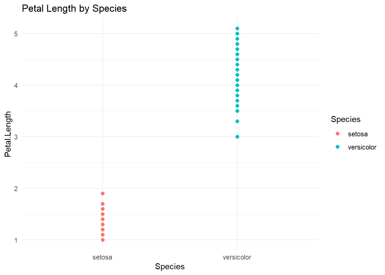

3.1.2 Check the Plot

ggplot(iris_two, aes(x = Species, y = Petal.Length, color = Species)) +
  geom_point(size = 2) +
  theme_minimal() +
  labs(title = "Petal Length by Species")

3.2 ANOVA

3.2.1 For more than two variables

anova_model <- aov(Petal.Length ~ Species, data = iris)
summary(anova_model)

##              Df Sum Sq Mean Sq F value Pr(>F)    
## Species       2  437.1  218.55    1180 <2e-16 ***
## Residuals   147   27.2    0.19                   
## ---
## Signif. codes:  0 '***' 0.001 '**' 0.01 '*' 0.05 '.' 0.1 ' ' 1

3.2.2 Pairwise comparisons (Tukey HSD)

TukeyHSD(anova_model)

##   Tukey multiple comparisons of means
##     95% family-wise confidence level
## 
## Fit: aov(formula = Petal.Length ~ Species, data = iris)
## 
## $Species
##                       diff     lwr     upr p adj
## versicolor-setosa    2.798 2.59422 3.00178     0
## virginica-setosa     4.090 3.88622 4.29378     0
## virginica-versicolor 1.292 1.08822 1.49578     0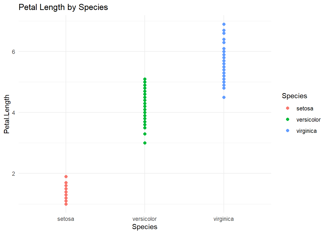

3.2.3 Check the Plot

ggplot(iris, aes(x = Species, y = Petal.Length, color = Species)) +
  geom_point(size = 2) +
  theme_minimal() +
  labs(title = "Petal Length by Species")

3.3 Correlation

cor.test(iris$Petal.Length, iris$Petal.Width)

## 
##  Pearson's product-moment correlation
## 
## data:  iris$Petal.Length and iris$Petal.Width
## t = 43.387, df = 148, p-value < 2.2e-16
## alternative hypothesis: true correlation is not equal to 0
## 95 percent confidence interval:
##  0.9490525 0.9729853
## sample estimates:
##       cor 
## 0.9628654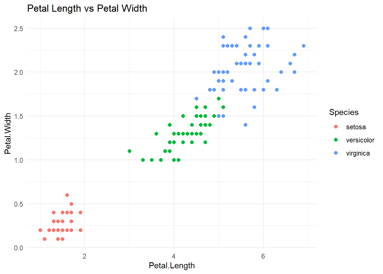

3.3.1 Check the Plot

ggplot(iris, aes(x = Petal.Length, y = Petal.Width, color = Species)) +
  geom_point(size = 2) +
  theme_minimal() +
  labs(title = "Petal Length vs Petal Width")

4 Build Your Own Graph

5 Session Info

Sys.time()

## [1] "2026-04-25 21:49:59 PDT"

sessionInfo()

## R version 4.5.1 (2025-06-13 ucrt)
## Platform: x86_64-w64-mingw32/x64
## Running under: Windows 11 x64 (build 26200)
## 
## Matrix products: default
##   LAPACK version 3.12.1
## 
## locale:
## [1] LC_COLLATE=English_United States.utf8 
## [2] LC_CTYPE=English_United States.utf8   
## [3] LC_MONETARY=English_United States.utf8
## [4] LC_NUMERIC=C                          
## [5] LC_TIME=English_United States.utf8    
## 
## time zone: America/Los_Angeles
## tzcode source: internal
## 
## attached base packages:
## [1] stats     graphics  grDevices utils     datasets  methods   base     
## 
## other attached packages:
##  [1] RColorBrewer_1.1-3 viridis_0.6.5      viridisLite_0.4.2  here_1.0.1        
##  [5] ggplot2_4.0.1      gt_1.1.0           gtsummary_2.5.0    tibble_3.3.0      
##  [9] purrr_1.1.0        dplyr_1.1.4        readxl_1.4.5      
## 
## loaded via a namespace (and not attached):
##  [1] sass_0.4.10       generics_0.1.4    tidyr_1.3.1       xml2_1.4.0       
##  [5] lattice_0.22-7    digest_0.6.37     magrittr_2.0.3    evaluate_1.0.5   
##  [9] grid_4.5.1        cards_0.7.1       fastmap_1.2.0     Matrix_1.7-3     
## [13] cellranger_1.1.0  rprojroot_2.1.1   jsonlite_2.0.0    gridExtra_2.3    
## [17] mgcv_1.9-3        scales_1.4.0      jquerylib_0.1.4   cli_3.6.5        
## [21] rlang_1.1.6       litedown_0.7      splines_4.5.1     commonmark_2.0.0 
## [25] withr_3.0.2       cachem_1.1.0      yaml_2.3.10       tools_4.5.1      
## [29] vctrs_0.6.5       R6_2.6.1          lifecycle_1.0.5   fs_1.6.6         
## [33] pkgconfig_2.0.3   pillar_1.11.0     bslib_0.9.0       gtable_0.3.6     
## [37] glue_1.8.0        xfun_0.53         tidyselect_1.2.1  rstudioapi_0.17.1
## [41] knitr_1.50        dichromat_2.0-0.1 farver_2.1.2      nlme_3.1-168     
## [45] htmltools_0.5.8.1 rmarkdown_2.29    labeling_0.4.3    compiler_4.5.1   
## [49] S7_0.2.0          markdown_2.0

Learning R through IRIS

USC Biomedical Student Research Seminar

Jonathan Nelson

25 April, 2026

1 Introduction

1.1 Download this .Rmd file

1.2 Read in the dataset

1.3 Inspect the data

1.4 Check the Structure

1.5 Get a Summary

2 Basic `dplyr` summaries

2.1 Count number of entries by Species

2.1.1 Compute average measurements by species

2.2 Filter rows

2.2.1 Look only at `setosa`

2.2.2 Look only at flowers with large petals

2.3 Create new variables

2.3.1 Create and Summarize

2.4 First ggplot: a scatterplot

2.4.1 Color by species

2.4.1.1 Color palette = `RColorBrewer`

2.4.1.2 Colorblind-friendly = `viridis`

2.5 Multidimensional Plots

2.5.1 Going 4D!

2.6 Faceting for comparison

2.7 Summaries plus plots

2.7.1 Calculate the Summary

2.7.2 Plot the Summary

3 Statistics

3.1 t-test

3.1.1 Filter to two variables

3.1.2 Check the Plot

3.2 ANOVA

3.2.1 For more than two variables

3.2.2 Pairwise comparisons (Tukey HSD)

3.2.3 Check the Plot

3.3 Correlation

3.3.1 Check the Plot

4 Build Your Own Graph

5 Session Info

Learning R through IRIS

USC Biomedical Student Research Seminar

Jonathan Nelson

25 April, 2026

1 Introduction

1.1 Download this .Rmd file

1.2 Read in the dataset

1.3 Inspect the data

1.4 Check the Structure

1.5 Get a Summary

2 Basic dplyr summaries

2.1 Count number of entries by Species

2.1.1 Compute average measurements by species

2.2 Filter rows

2.2.1 Look only at setosa

2.2.2 Look only at flowers with large petals

2.3 Create new variables

2.3.1 Create and Summarize

2.4 First ggplot: a scatterplot

2.4.1 Color by species

2.4.1.1 Color palette = RColorBrewer

2.4.1.2 Colorblind-friendly = viridis

2.5 Multidimensional Plots

2.5.1 Going 4D!

2.6 Faceting for comparison

2.7 Summaries plus plots

2.7.1 Calculate the Summary

2.7.2 Plot the Summary

3 Statistics

3.1 t-test

3.1.1 Filter to two variables

3.1.2 Check the Plot

3.2 ANOVA

3.2.1 For more than two variables

3.2.2 Pairwise comparisons (Tukey HSD)

3.2.3 Check the Plot

3.3 Correlation

3.3.1 Check the Plot

4 Build Your Own Graph

5 Session Info

2 Basic `dplyr` summaries

2.2.1 Look only at `setosa`

2.4.1.1 Color palette = `RColorBrewer`

2.4.1.2 Colorblind-friendly = `viridis`